Interaction graphs and signed system changes
This is work in progress! The content is still incomplete and changing.
In this first part of the Sign Consistency Methods (SCM) series, we will introduce interaction graph models and how they are used by SCM to model the changes in a dynamic system.
What are interaction graphs?
Interaction or influence graphs are a widely-used representation for complex systems. The components or variables of the system are represented by nodes, and edges denote how these components interact with each other. Many biological systems have a representation as interaction graphs, such as hunter-prey models, gene regulatory networks, and signaling networks.
A more formal definition of an interaction graph is as follows:
Definition 1: An interaction graph is a signed directed graph (V, E, σ), where V is a set of nodes that represent system variables, E is a set of edges that represent the influence of changes in one variable on another, and σ : E → {+, –} is a labeling of the edges that indicates whether the change in one variable tends to increase or decrease the value of another variable.
An edge i→j in the graph indicates that the change in the value of variable i has an influence on the value of variable j, and the sign label σ(i,j) specifies whether this influence is positive (i tends to increase j) or negative (i tends to decrease j).
An example of an interaction graph is given in Figure 1. There exist many variants of interaction graphs, some have weighted edges and some have other kinds of edges or different types of nodes. But this definition will suffice for now.
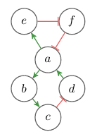
Fig. 1: Example of an interaction graph. Green arrows indicate positive (+) influence, red edges negative (–) influence.
What are signed system changes?
Interaction graphs are models of dynamic quantitative systems where a quantitative state of the system is a mapping Si : V → ℝ+. Sign consistency methods use signs to denote changes in the variables of the modeled system. Examples for such changes could be increase or decrease in metabolite concentrations or expression levels of genes. The signs + and – are used to denote increase and decrease and 0 signifies no-change. Sign consistency methods relate the IG model of the system and the variations between system states by representing the variations as labels on the nodes in the graph. For example, the changes between two states of the system are represented by labeling the nodes of IG with the signs of the change in the corresponding system variable. Given two system states SR and SO the differences between these states can be represented as the labeling μRO : V →{+,–,0} with μRO(x) = sign(xSO - xSR). See Figure 2 for an example of two states and the corresponding sign labeling. We use the colors , , to represent the signs +, –, 0.
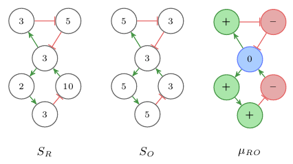
Fig. 2: Example of a sign labeling representing the changes between two quantitative states.
Sign consistency rules
Sign consistency methods define rules that determine which labelings of the graph are considered consistent and which are considered inconsistent. There exist several different consistency rules which are useful to model different properties of a biological system. For now we only consider the following.
Rule 1 (backwards propagation) Every change in a node must be explained by a change in one of its predecessors. Let (V,E,σ) be an IG. Then a labeling μ : V →{+,–,0} satisfies Rule 1 for node i ∈ V iff
- μ(i) = 0, or
- there is some edge j→i in E such that μ(i) = μ(j)σ(j,i).
Rule 1 implements backward reasoning. Given an effect we look backwards to verify its cause. Labelings that are consistent with this rule represent the differences between steady states. In a steady state the values of all state variables are balanced. Hence, the change in one variable must be sustained by the change in one of its predecessors. In other words, if SR and SO are steady states of the system then the labeling μRO is consistent with Rule 1. The trivial example is when both states are the same SR = SO then nothing changes ∀x ∈ V : μRO(x) = 0.
Let’s see what else we can do with that. Figure 3 shows an interaction graph and all labelings μi : V →{+,–,0} with μi(a) = + that satisfy Rule 1.
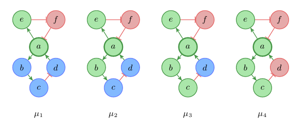
Fig. 3: Labeled interaction graph
Often it is useful to represent the labelings in a table as shown in Table 1. As you can see, there exist only four labelings that satisfy these constraints. In every of these labeling it holds μi(e) = + and μi(f) = –. We can use this table to predict the behavior of the system. We see that in every steady state, with an increase in a we also have an increase in e and a decrease in f. For b and c we can predict that they will not decrease, and for d that it will not increase.
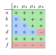
Table 1: Table of admissible labelings.
Conclusion
In this part I introduced interaction graphs and explained how they can be used to model biological systems. We have seen how sign consistency methods represent variations in the system as sign labelings, and how sign consistency constraints can be used to derive predictions over the steady states of a system. So far we have modeled a closed system. In Part 2 I will introduce external inputs and perturbations.