Predicting effects on downstream regulated variables
This is work in progress! The content is still incomplete and changing.
This is Part 4 of the sign consistency series. Previously, we covered the sign consistency rule for backward propagation which works for transitions between steady states. In this part I introduce another consistency rule that also works for steady state transitions, and increases the predictive power of sign consistency methods.
Forward propagation
The backward reasoning implemented by Rule 1 is very cautious. It expresses the assumption is that for every effect there must be a cause but it excludes the assumption that a change must have and effect. Figure 1 shows all labelings μi that are consistent with Rule 1 and were μi(b) = +. In all labelings it holds that μi(a) = +, so we can predict very precisely the cause for an increase in b. But the labelings for c are ambiguous, although we see an increase in b we cannot predict an increase in c.
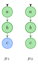
Fig. 1: Prediction under consistency Rule 1. Backward propagation does not allow an unambiguous prediction for c.
To increase the predictive power of our method we define a new consistency rule that implements the assumption that a change in one variable has an effect on its successors. We define this rule for independent regulations i → j were a change in i is sufficient to cause an change in j. In the next part we will introduce cooperative (dependent) regulations were it depends on other variables in the system whether the change in i will have an effect on j.
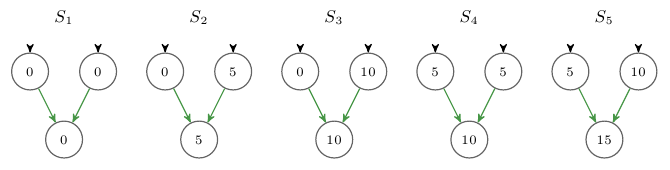
Fig. 2: Five quantitative stable states of a variable with two independent regulations.
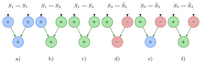
Fig. 3: Sign labeling representation of possible transitions among the states in Figure 2. The ~ means that the values of the input nodes have been switched left to right in the state.
Figure 2 shows exemplarily five quantitative representations of stable states of a system were one variable is independently regulated by two predecessors. In Figure 3 we see the possible sign labelings representing different state transitions. We see that for the cases a-c there exists an unambiguous input output behavior. In the cases d-f we see different outputs for the same input. This behavior is enforced through the following forward propagation rule.
Rule 3 (forward propagation) 0-change can only occur in a variable that does not depend on other variables with change, or if it receives opposing regulations.
Let (V,E,σ) be an IG. Then a labeling μ : V →{+,–,0} satisfies Rule 3 for node i ∈ V iff
- μ(i)≠0, or
- there is no edge j → i in E such that μ(j)σ(j,i) ∈{+,–}, or
- there exist at least two edges j1 → i and j2 → i in E such that μ(j1)σ(j1,i)+ μ(j2)σ(j2,i) = 0.
This rule implements forward propagation by restricting the occurrence of 0. In other words Rule 3 limits the cases were a change in an upstream node can have no effect on the regulated down stream node. We can see now that labeling μ1 in Figure 1 does not satisfy Rule 3 for c. Only labeling μ2 satisfies both Rule 1 and 3 for all nodes, leaving us with only one possible behavior.
Conclusion
In this part I have introduced the forward propagation rule for independent regulations, and we have seen how forward propagation increases the predictive power of sign consistency methods. In the next part I will show how we can implement forward propagation for cooperative (dependent) regulations.