Modeling open systems inputs and perturbations
This is work in progress! The content is still incomplete and changing.
This is Part 2 of the sign consistency series. In Part 1 of this series we learned how to use interaction graphs and sign consistency methods to reason about steady states in closed systems. In this part we add inputs to our model and answer the question how a biological system responds to external influences.
Inputs and perturbations
Most systems interact in some ways with a surrounding environment. To reason over systems response to different environmental settings we introduce input variables. Input variables are not controlled by the system but represent external influences on the system. Such inputs could be stressors like temperature, light or drugs. In an IG (E,V) we denote the set of nodes that represent input variables with I ⊆ V. Because input nodes are controlled externally, they are excluded from the sign consistency rules.
For the closed system shown in Figure 1, there exists no single labeling μ : V→{+,–,0}, with μ(a) = + and μ(b) = – that satisfies Rule 1 for all v ∈ V. In other words, there exists no transition between steady states where a increases and b decreases. Because a is the only predecessor of b, between all steady states changes in a and b must have the same sign.
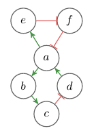
Fig. 1: Example of an interaction graph. Green arrows indicate positive (+) influence, red edges negative (–) influence.
We can interpret our model as an open system, were the value of b is determined by the environment by declaring b as input variable. With perturbations we can now take control over the input variables and find out how the system behaves under different environmental conditions. For example we can now find out how our system reacts to a decrease in b. Figure 2 shows all labelings μi that satisfy Rule 1 for all v ∈ V \ I with I = {b} and μi(a) = + and μi(b) = –. Input nodes are denoted with a black incoming arrow.

Fig. 2: Labeled interaction graph
We see that using a perfect perturbation, a sustained decrease of b, the system can reach a quasi steady state where both a and d are increased. This is a state which could not be reached in the closed system without perturbation. While this is already an interesting reasoning mode, it is even more interesting to flip the question around and use this approach to do some treatment planning. Let’s see, what are the minimal perturbations that would allow the system to transition into a state where a and d are increased? Figure 3 shows the potential perturbations (along with partial labelings) that allow for such a state-transition. We can see that we have two more alternatives to reach our goal, either a direct increase in d or a decrease in c.
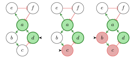
Fig. 3: Minimal perturbations of the system that can results in an increase of a and d (along with partial labeling)
Perturbations and model topology
Perturbations play a major role in the analysis of biological models. A complementary view point on perturbations is that they allow us to alter the model structure. In particular, all incoming edges of an input node can be ignored because the node is no longer constrained by the system but by us. A special role play so called 0-perturbations, these are perturbations were the value of a variable is kept constant over the state transition. For those nodes the only possible label is 0 and we can ignore their outgoing edges because they can’t be responsible for any downstream changes. It’s easy to see that for complex models with many cyclic interactions such perturbations are very useful to investigate the influence of single components while excluding the influence of others. In a later part, we will see how perturbations are used to design experiments that allow to discriminate among alternative model topologies.
Conclusion
In this part I introduced inputs and we have seen how one can model perturbations of a system. We have seen how we can reason over possible perturbations of a systems, and how to use this for treatment planning. In the next part I will introduce a new consistency rule that allows us to handle constraints that are posed by the minima and maxima of the system variables.